Dosiero:Bloop locations.png
Grandeco de ĉi antaŭvido: 600 × 600 rastrumeroj. Aliaj distingivoj: 240 × 240 rastrumeroj | 480 × 480 rastrumeroj | 768 × 768 rastrumeroj | 1 024 × 1 024 rastrumeroj | 2 048 × 2 048 rastrumeroj | 3 000 × 3 000 rastrumeroj.
Bildo en pli alta difino ((3 000 × 3 000 rastrumeroj, grandeco de dosiero: 7,74 MB, MIME-tipo: image/png))
| Jen dosiero de la Wikimedia-Komunejo. La priskribo en ties priskriba paĝo estas montrata suben.
|
Resumo
| Priskribo |
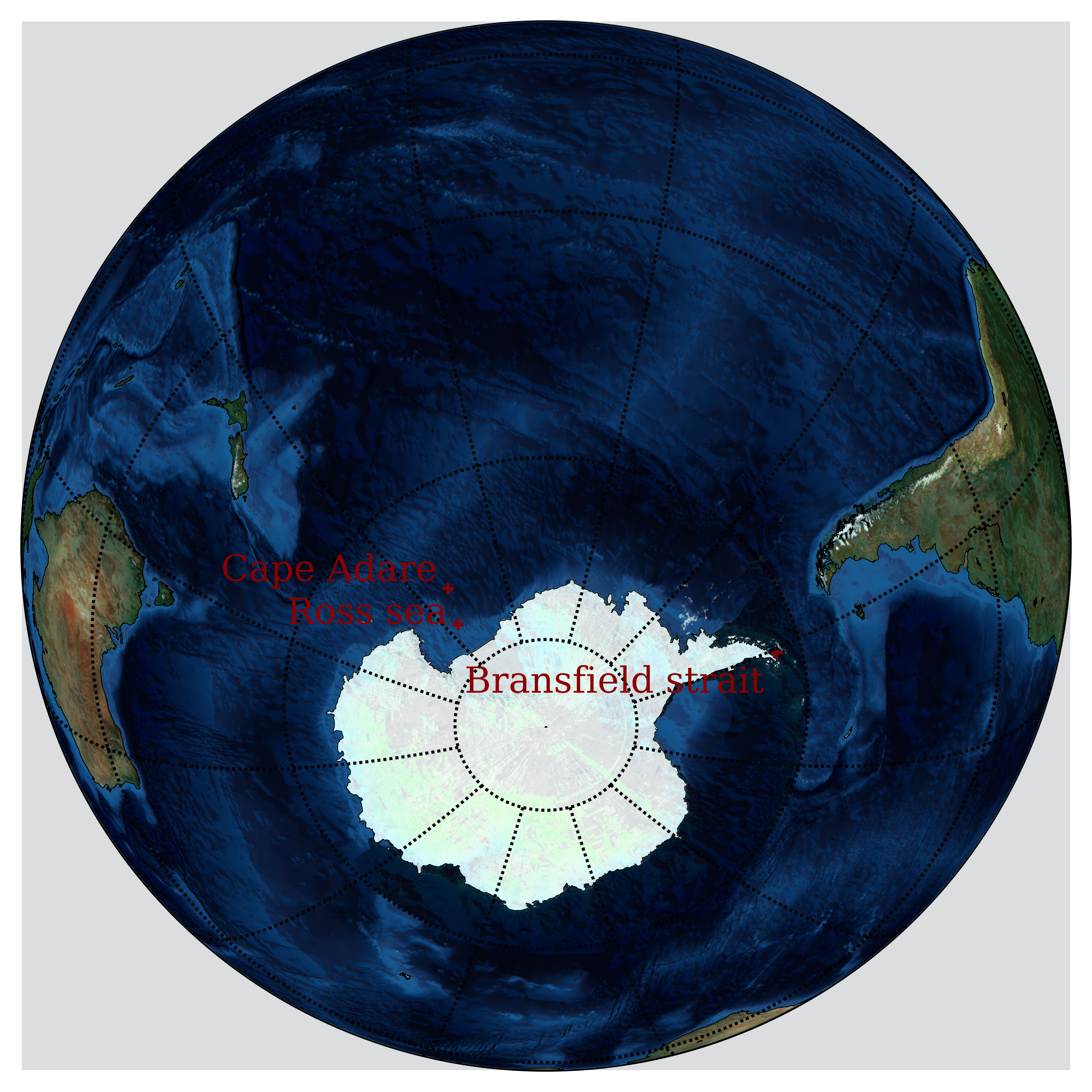
English: Possible locations of the Bloop, an ultra-low frequency and extremely powerful underwater sound detected by the U.S. National Oceanic and Atmospheric Administration (NOAA) in 1997. |
| Dato | |
| Fonto | Propra verko |
| Aŭtoro | Nojhan |
| PNG genesis |
Source code
This image has been generated by the following source code in Python:
Python code
| source code |
|---|
print "import modules...",
import sys
sys.stdout.flush()
import pickle
from mpl_toolkits.basemap import Basemap, shiftgrid, cm
import matplotlib
import matplotlib.pyplot as plt
import numpy as np
from netCDF4 import Dataset
print "ok"

# Lovecraft: 47:9'S 126:43'W
# lovecraft_lat = -47.9
# lovecraft_lon = -126.43

# August Derleth: 49:51'S 128:34'W
# derleth_lat = -49.51
# derleth_lon = -128.34

# Nemo point: 48:52.6'S 123:23.6'W
# nemo_lat = -48.526
# nemo_lon = -123.236

# The Bloop:
bransfield_strait_lat=-63
bransfield_strait_lon=-59
ross_sea_lat = -75
ross_sea_lon = -175
cape_adare_lat = -71.17
cape_adare_lon = -170.14

mid_lat = np.mean((bransfield_strait_lat,ross_sea_lat,cape_adare_lat))
mid_lon = np.mean((bransfield_strait_lon,ross_sea_lon,cape_adare_lon))


# Not necessary, because the default projection is ortho,
# but can be useful if you want another one.
def equi(m, centerlon, centerlat, radius, *args, **kwargs):
    """
    Drawing circles of a given radius around any point on earth, given the current projection.
    http://www.geophysique.be/2011/02/20/matplotlib-basemap-tutorial-09-drawing-circles/
    """
    glon1 = centerlon
    glat1 = centerlat
    X = []
    Y = []
    for azimuth in range(0, 360):
        glon2, glat2, baz = shoot(glon1, glat1, azimuth, radius)
        X.append(glon2)
        Y.append(glat2)
    X.append(X[0])
    Y.append(Y[0])

    #m.plot(X,Y,**kwargs) #Should work, but doesn't...
    X,Y = m(X,Y)
    plt.plot(X,Y,**kwargs)


def shoot(lon, lat, azimuth, maxdist=None):
    """Shooter Function
    Plotting great circles with Basemap, but knowing only the longitude,
    latitude, the azimuth and a distance. Only the origin point is known.
    Original javascript on http://williams.best.vwh.net/gccalc.htm
    Translated to python by Thomas Lecocq :
    http://www.geophysique.be/2011/02/19/matplotlib-basemap-tutorial-08-shooting-great-circles/
    """
    glat1 = lat * np.pi / 180.
    glon1 = lon * np.pi / 180.
    s = maxdist / 1.852
    faz = azimuth * np.pi / 180.

    EPS= 0.00000000005
    if ((np.abs(np.cos(glat1))<EPS) and not (np.abs(np.sin(faz))<EPS)):
        alert("Only N-S courses are meaningful, starting at a pole!")

    a=6378.13/1.852
    f=1/298.257223563
    r = 1 - f
    tu = r * np.tan(glat1)
    sf = np.sin(faz)
    cf = np.cos(faz)
    if (cf==0):
        b=0.
    else:
        b=2. * np.arctan2 (tu, cf)

    cu = 1. / np.sqrt(1 + tu * tu)
    su = tu * cu
    sa = cu * sf
    c2a = 1 - sa * sa
    x = 1. + np.sqrt(1. + c2a * (1. / (r * r) - 1.))
    x = (x - 2.) / x
    c = 1. - x
    c = (x * x / 4. + 1.) / c
    d = (0.375 * x * x - 1.) * x
    tu = s / (r * a * c)
    y = tu
    c = y + 1
    while (np.abs (y - c) > EPS):

        sy = np.sin(y)
        cy = np.cos(y)
        cz = np.cos(b + y)
        e = 2. * cz * cz - 1.
        c = y
        x = e * cy
        y = e + e - 1.
        y = (((sy * sy * 4. - 3.) * y * cz * d / 6. + x) *
              d / 4. - cz) * sy * d + tu

    b = cu * cy * cf - su * sy
    c = r * np.sqrt(sa * sa + b * b)
    d = su * cy + cu * sy * cf
    glat2 = (np.arctan2(d, c) + np.pi) % (2*np.pi) - np.pi
    c = cu * cy - su * sy * cf
    x = np.arctan2(sy * sf, c)
    c = ((-3. * c2a + 4.) * f + 4.) * c2a * f / 16.
    d = ((e * cy * c + cz) * sy * c + y) * sa
    glon2 = ((glon1 + x - (1. - c) * d * f + np.pi) % (2*np.pi)) - np.pi

    baz = (np.arctan2(sa, b) + np.pi) % (2 * np.pi)

    glon2 *= 180./np.pi
    glat2 *= 180./np.pi
    baz *= 180./np.pi

    return (glon2, glat2, baz)


print "read in etopo5 topography/bathymetry"
url = 'http://ferret.pmel.noaa.gov/thredds/dodsC/data/PMEL/etopo5.nc'
etopodata = Dataset(url)

print "get data"

def topopickle(etopodata,name):
    import sys
    print "\t"+name+"...",
    sys.stdout.flush()
    filename = "rlyeh_"+name+".pickle"
    try:
        with open(filename,"r") as fd:
            print "load...",
            var = pickle.load(fd)
    except IOError:
        print "copy...",
        var = etopodata.variables[name][:]
        with open(filename,"w") as fd:
            print "dump...",
            pickle.dump(var,fd)
    print "ok"
    return var

topoin = topopickle(etopodata,"ROSE")
lons   = topopickle(etopodata,"ETOPO05_X")
lats   = topopickle(etopodata,"ETOPO05_Y")
print "shift data so lons go from -180 to 180 instead of 20 to 380...",
sys.stdout.flush()
topoin,lons = shiftgrid(180.,topoin,lons,start=False)
print "ok"


# create the figure and axes instances.
fig = plt.figure()
ax = fig.add_axes([0.1,0.1,0.8,0.8])

print "setup basemap"
# set up orthographic m projection with
# perspective of satellite looking down at 50N, 100W.
# use low resolution coastlines.
m = Basemap(projection='ortho',lat_0=mid_lat,lon_0=mid_lon,resolution='l')
m.bluemarble()

# Generic Mapping Tools colormaps:
# GMT_drywet, GMT_gebco, GMT_globe, GMT_haxby GMT_no_green, GMT_ocean, GMT_polar,
# GMT_red2green, GMT_relief, GMT_split, GMT_wysiwyg

print "transform to nx x ny regularly spaced native projection grid"
# step=5000.
step=10000.
nx = int((m.xmax-m.xmin)/step)+1; ny = int((m.ymax-m.ymin)/step)+1
topodat = m.transform_scalar(topoin,lons,lats,nx,ny)

print "plot topography/bathymetry as shadows"
from matplotlib.colors import LightSource
ls = LightSource(azdeg = 45, altdeg = 220, hsv_min_val=0.0, hsv_max_val=1.0,
        hsv_min_sat=0.0, hsv_max_sat=1.0)
# convert data to rgb array including shading from light source.
# (must specify color m)
rgb = ls.shade(topodat, cm.GMT_ocean)
im = m.imshow(rgb, alpha=0.15)

print "draw coastlines, country boundaries, fill continents"
m.drawcoastlines(linewidth=0.25)
# draw the edge of the map projection region
m.drawmapboundary(fill_color='white')
# draw lat/lon grid lines every 30 degrees.
m.drawmeridians(np.arange(  0,360,30), color="black" )
m.drawparallels(np.arange(-90,90 ,30), color="black" )

print "draw points"
psize=5
font = {'family' : 'serif',
        'weight' : 'normal',
        'size'   : 12}
matplotlib.rc('font', **font)

# x,y = m( lovecraft_lon, lovecraft_lat )
# m.scatter(x,y,psize,marker='o', color='white')
# plt.text(x+50000,y+50000+50000, "Lovecraft", color='white')
#
# x,y = m( derleth_lon, derleth_lat )
# m.scatter(x,y,psize,marker='o',color='white')
# plt.text(x+50000-120000,y+50000, "Derleth", color='white', horizontalalignment="right")

# x,y = m( nemo_lon, nemo_lat )
# m.scatter(x,y,psize*3,marker='+',color='#555555')
# plt.text(x+50000+50000,y+50000-80000, "Nemo", color="#555555", verticalalignment="top")
#
# equi(m, nemo_lon, nemo_lat, radius=2688, color="#555555" )

pcolor="darkred"
offset=150000

x,y = m( bransfield_strait_lon, bransfield_strait_lat )
m.scatter(x,y,psize*3,marker='+',color=pcolor)
plt.text(x-offset,y-offset, "Bransfield strait", color=pcolor,
        horizontalalignment="right", verticalalignment="top")

x,y = m( ross_sea_lon, ross_sea_lat )
m.scatter(x,y,psize*3,marker='+',color=pcolor)
plt.text(x-offset,y, "Ross sea", color=pcolor,
        horizontalalignment="right", verticalalignment="bottom")

x,y = m( cape_adare_lon, cape_adare_lat )
m.scatter(x,y,psize*3,marker='+',color=pcolor)
plt.text(x-offset,y, "Cape Adare", color=pcolor,
        horizontalalignment="right", verticalalignment="bottom")

plt.savefig("Bloop_locations.png", dpi=600, bbox_inches='tight')
# plt.show()
|
Permesiloj:
Mi, la posedanto de la aŭtorrajto por ĉi tiu verko, ĉi-maniere publikigas tiun laŭ la jena permesilo:
Ĉi tiu dosiero estas disponebla laŭ la permesilo Krea Komunaĵo Atribuite-Samkondiĉe 3.0 Neadaptita.
- Vi rajtas:
- kunhavigi – kopii, distribui kaj publikigi la verkon
- aliigi – modifi, adapti, kompletigi, transformi, uzi la tutan verkon aŭ ties partojn, memstare aŭ en aliaj verkoj
- La verko rajtas esti kunhavigata nur:
- atribuite – Vi devas atribui aŭtorecon, liveri ligilon al la permesilo kaj marki ĉu ŝanĝoj estis faritaj. Faru tion en aprobinda maniero, tamen ne sugestante, ke permesinto aprobas vin aŭ vian uzon.
- samkondiĉe – Se vi rekombinas la verkon, transformas ĝin aŭ kreas devenaĵon bazitan sur ĝi, vi rajtas distribui la rezultan verkon nur laŭ la sama aŭ kongrua permesilo kompare kun ĉi tiu.
Dosierhistorio
Alklaku iun daton kaj horon por vidi kiel la dosiero tiam aspektis.
| Dato/Horo | Bildeto | Grandecoj | Uzanto | Komento | |
|---|---|---|---|---|---|
| nun | 21:46, 12 feb. 2013 | | 3 000 × 3 000 (7,74 MB) | Nojhan | User created page with UploadWizard |
Dosiera uzado
La jena paĝo ligas al ĉi tiu dosiero:
Suma uzado de la dosiero
La jenaj aliaj vikioj utiligas ĉi tiun dosieron:
- Uzado en de.wikipedia.org
- Uzado en es.wikipedia.org
- Uzado en fr.wikipedia.org
- Uzado en id.wikipedia.org
- Uzado en it.wikipedia.org